Expected Output: 02_spectrum
This document shows the expected console output and example figures from all examples in python/src/adctoolbox/examples/02_spectrum/.
Summary
All examples in 02_spectrum demonstrate spectrum analysis capabilities:
exp_s01-s03: Basic spectrum analysis (simplest, interactive, save figure)
exp_s04: Dynamic range sweep
exp_s05: Harmonic spur annotation
exp_s06: FFT length and OSR sweep
exp_s07: Power vs coherent averaging
exp_s08: Windowing functions comparison (Kaiser, Blackman-Harris, Hann, Hamming)
exp_s10: Polar spectrum - thermal noise vs harmonic distortion
exp_s11: Polar spectrum - static nonlinearity vs memory effect
exp_s12: Polar spectrum - coherent averaging improvement
exp_s21: Two-tone spectrum analysis with IMD products
exp_s22: Two-tone IMD comparison (weak vs strong nonlinearity)
exp_s23: Two-tone coherent averaging
Total Examples: 14
exp_s01_analyze_spectrum_simplest.py
Description: Simplest example - analyze spectrum with minimal code.
[Nonideal] Noise RMS=[10.00 uVrms], Theoretical SNR=[90.97 dB], Theoretical NSD=[-167.96 dBFS/Hz]

[analyze_spectrum] ENoB=[14.80 b], SNDR=[90.89 dB], SFDR=[115.33 dB], SNR=[90.90 dB], NSD=[-167.89 dBFS/Hz]
exp_s02_analyze_spectrum_interactive.py
Description: Interactive example - displays plot window.
[Sinewave] Fs=[100.00 MHz], Fin=[12.00 MHz], Bin/N=[983/8192], A=[0.500 Vpeak]
[Nonideal] Noise RMS=[50.00 uVrms], Theoretical SNR=[76.99 dB], Theoretical NSD=[-153.98 dBFS/Hz]

[analyze_spectrum] ENoB=[12.51 b], SNDR=[77.08 dB], SFDR=[100.37 dB], SNR=[77.10 dB], NSD=[-154.09 dBFS/Hz]

[Figure displayed - close the window to exit]
exp_s03_analyze_spectrum_savefig.py
Description: Save figure to file instead of displaying.
[Sinewave] Fs=[100.00 MHz], Fin=[12.00 MHz], Bin/N=[983/8192], A=[0.500 Vpeak]
[Nonideal] Noise RMS=[200.00 uVrms], Theoretical SNR=[64.95 dB], Theoretical NSD=[-141.94 dBFS/Hz]

[analyze_spectrum] ENoB=[10.50 b], SNDR=[ 64.97 dB], SFDR=[ 88.02 dB], SNR=[ 64.98 dB], NSD=[-141.97 dBFS/Hz]
[analyze_spectrum] Noise Floor=[ -64.98 dBFS], Signal Power=[  0.00 dBFS] (expected: 0.00 dB for 1.000V in 1.0V FSR),

[Sinewave] Fs=[100.00 MHz], Fin=[12.00 MHz], Bin/N=[983/8192], A=[0.250 Vpeak]
[Nonideal] Noise RMS=[200.00 uVrms], Theoretical SNR=[58.93 dB], Theoretical NSD=[-135.92 dBFS/Hz]

[analyze_spectrum] ENoB=[ 9.50 b], SNDR=[ 58.95 dB], SFDR=[ 82.51 dB], SNR=[ 58.96 dB], NSD=[-141.97 dBFS/Hz]
[analyze_spectrum] Noise Floor=[ -64.98 dBFS], Signal Power=[ -6.02 dBFS] (expected: -6.02 dB for 0.500V in 1.0V FSR),


[Save fig] -> [D:\ADCToolbox\python\src\adctoolbox\examples\02_spectrum\output\exp_s03_analyze_spectrum_savefig.png]
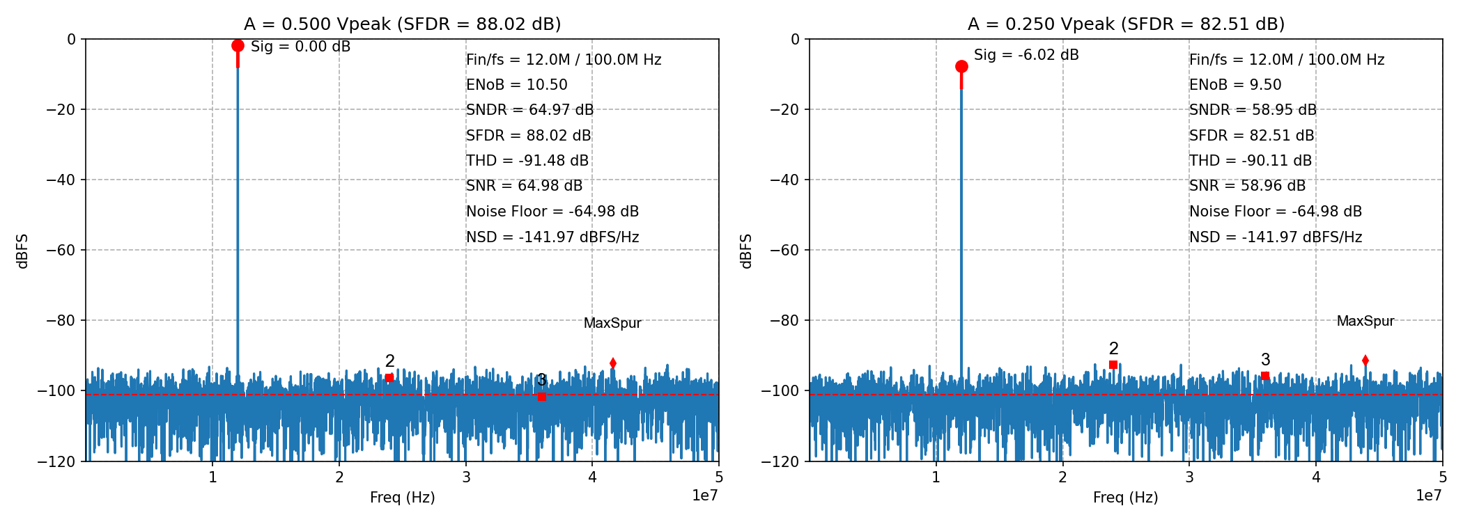
Basic FFT spectrum analysis with all key metrics
exp_s04_sweep_dynamic_range.py
Description: Sweep signal amplitude to characterize dynamic range.
[Sinewave] Fs=[100.00 MHz], Fin=[11.999512 MHz] (coherent, Bin 983), N=[8192]
[Nonideal] Noise RMS=[100.00 uVrms] (fixed)
[Sweep] Amplitude: -80.0 to 0.0 dBFS (50 steps)

================================================================================
DYNAMIC RANGE SWEEP
================================================================================
[A= -80.0 dBFS] SNR=[ -8.84 dB] (Theory: -9.0 dB), Noise Floor=[ -70.97 dBFS]
[A= -78.4 dBFS] SNR=[ -7.24 dB] (Theory: -7.4 dB), Noise Floor=[ -70.83 dBFS]
[A= -76.7 dBFS] SNR=[ -5.47 dB] (Theory: -5.8 dB), Noise Floor=[ -70.94 dBFS]
... (50 total steps)
[A=  -3.3 dBFS] SNR=[ 67.67 dB] (Theory: 67.7 dB), Noise Floor=[ -70.94 dBFS]
[A=  -1.6 dBFS] SNR=[ 69.30 dB] (Theory: 69.3 dB), Noise Floor=[ -70.94 dBFS]
[A=   0.0 dBFS] SNR=[ 70.86 dB] (Theory: 71.0 dB), Noise Floor=[ -70.86 dBFS]

[Save fig] -> [D:\ADCToolbox\python\src\adctoolbox\examples\02_spectrum\output\exp_s04_sweep_dynamic_range.png]


================================================================================
SUMMARY: Dynamic Range Analysis
================================================================================
Dynamic Range: -71.1 dBFS (SNR=0dB) to 0.0 dBFS (max) = 71.1 dB
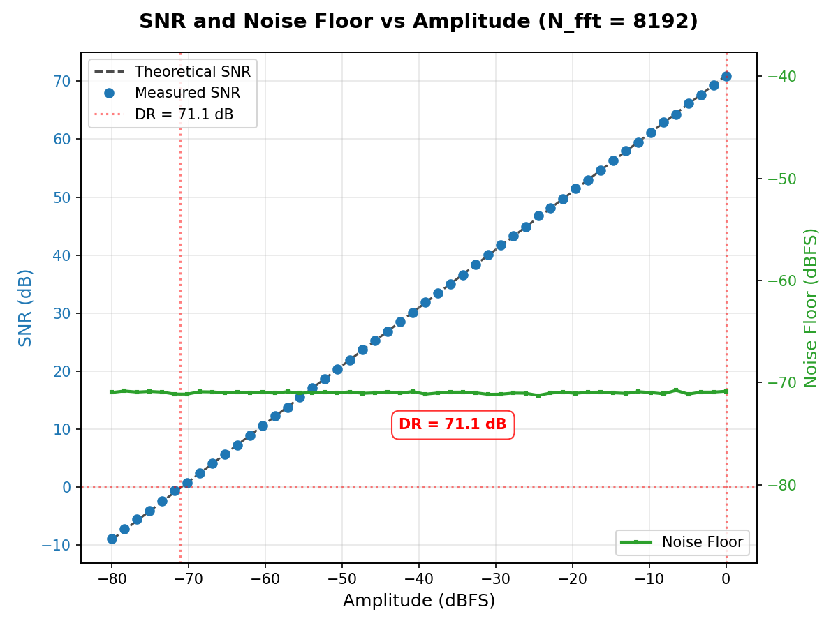
FFT metrics across input signal amplitudes (dynamic range sweep)
exp_s05_annotating_spur.py
Description: Annotate spur frequencies and demonstrate harmonic aliasing.
[Sinewave] Fs=[100.00 MHz], A=[0.500 Vpeak]
[Nonideal] HD2=[-100 dB], HD3=[-80 dB], Noise RMS=[50.00 uVrms], Theoretical SNR=[76.99 dB], Theoretical NSD=[-153.98 dBFS/Hz]

[Frequency 1] Fs/17.6 (No Collision): Fin=[5.68 MHz], Bin/N=[29789/524288], Harmonics spread
  [n_thd=11] ENoB=[12.20 b], SNDR=[ 75.20 dB], THD=[ -79.94 dB]

[Frequency 2] Fs/3: Fin=[33.33 MHz], Bin/N=[174763/524288], Collide at Nyquist!
[Warning from analyze_spectrum]: Harmonics [2, 4, 5, 7] alias to fundamental (excluded from THD)
  [n_thd=11] ENoB=[12.25 b], SNDR=[ 75.48 dB], THD=[ -80.79 dB]


[Save fig] -> [D:\ADCToolbox\python\src\adctoolbox\examples\02_spectrum\output\exp_s05_annotating_spur.png]
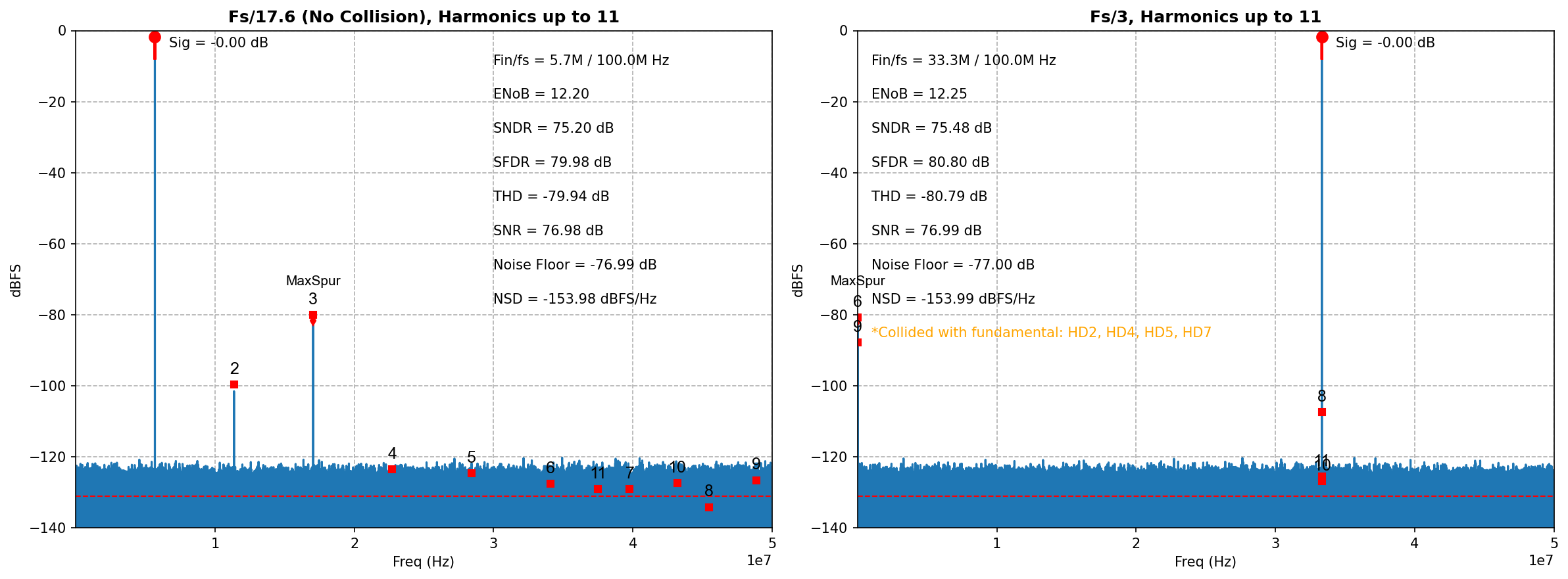
Spectrum with annotated fundamental, harmonics, and spurs
exp_s06_sweeping_fft_and_osr.py
Description: Compare FFT length vs OSR for improving spectrum quality.
[Sinewave] Fs=[100.00 MHz], A=[0.500 Vpeak]
[Nonideal] Noise RMS=[150.00 uVrms], Theoretical SNR=[67.45 dB], Theoretical NSD=[-144.44 dBFS/Hz]

================================================================================
SCENARIO 1: FFT LENGTH SWEEP (N = 2^7 to 2^16)
================================================================================
[N=     128 (2^ 7)] [Bin =  781.250 kHz] ENoB=[10.92 b], SNDR=[ 67.49 dB], SNR=[ 68.43 dB], NSD=[-145.42 dBFS/Hz]
[N=    1024 (2^10)] [Bin =   97.656 kHz] ENoB=[10.86 b], SNDR=[ 67.15 dB], SNR=[ 67.20 dB], NSD=[-144.19 dBFS/Hz]
[N=    8192 (2^13)] [Bin =   12.207 kHz] ENoB=[10.93 b], SNDR=[ 67.53 dB], SNR=[ 67.54 dB], NSD=[-144.54 dBFS/Hz]
[N=   65536 (2^16)] [Bin =    1.526 kHz] ENoB=[10.92 b], SNDR=[ 67.47 dB], SNR=[ 67.48 dB], NSD=[-144.47 dBFS/Hz]

================================================================================
SCENARIO 2: OVERSAMPLING RATIO SWEEP (OSR = 1, 2, 4, 10)
================================================================================
[Sinewave] Fin=[0.099182 MHz] (coherent, Bin 65), N=[65536]
[OSR=  1] ENoB=[10.91 b], SNDR=[ 67.45 dB], SNR=[ 67.45 dB], NSD=[-144.45 dBFS/Hz], Gain=[+0.0 dB] (Theory: +0.0 dB)
[OSR=  2] ENoB=[11.42 b], SNDR=[ 70.49 dB], SNR=[ 70.49 dB], NSD=[-144.47 dBFS/Hz], Gain=[+3.0 dB] (Theory: +3.0 dB)
[OSR=  4] ENoB=[11.91 b], SNDR=[ 73.48 dB], SNR=[ 73.48 dB], NSD=[-144.46 dBFS/Hz], Gain=[+6.0 dB] (Theory: +6.0 dB)
[OSR= 10] ENoB=[12.56 b], SNDR=[ 77.38 dB], SNR=[ 77.39 dB], NSD=[-144.39 dBFS/Hz], Gain=[+9.9 dB] (Theory: +10.0 dB)

[Save fig] -> [D:\ADCToolbox\python\src\adctoolbox\examples\02_spectrum\output\exp_s06_sweeping_fft_and_osr.png]

================================================================================
SUMMARY: FFT Length vs OSR
================================================================================
1. FFT Length (N):
   - Increases frequency resolution (bin width = Fs/N)
   - Lowers noise floor per bin (NSD improves)
   - Does NOT improve SNR (noise bandwidth unchanged)
   - Use case: Resolve closely spaced frequency components

2. Oversampling Ratio (OSR):
   - Directly improves SNR: Measured gain = +9.9 dB for OSR=10
   - Theoretical gain: +10.0 dB (10*log10(10))
   - Narrows analysis bandwidth to Fs/(2*OSR)
   - Use case: Delta-Sigma ADCs, narrowband signal analysis

3. Practical Guidelines:
   - For resolving harmonics: Increase FFT length
   - For improving SNR: Increase OSR (if signal is narrowband)
   - For best results: Combine both (large N + appropriate OSR)
exp_s07_spectrum_averaging.py
Description: Compare power averaging vs coherent averaging.
[Sinewave] Fs=[100.00 MHz], Fin=[4.992676 MHz] (coherent, Bin 409), N=[8192], A=[0.499 Vpeak]
[Nonideal] HD2=[-100 dB], HD3=[-90 dB], Noise RMS=[100.00 uVrms], Theoretical SNR=[70.95 dB], Theoretical NSD=[-147.94 dBFS/Hz]

[Generated] 100 runs with random phase

================================================================================
POWER SPECTRUM AVERAGING vs COHERENT SPECTRUM AVERAGING
================================================================================
[  1 Run(s)] Power Avg: ENoB=[11.49 b], SNR=[ 71.02 dB] | Coherent Avg: ENoB=[11.49 b], SNR=[ 71.02 dB]
[ 10 Run(s)] Power Avg: ENoB=[11.49 b], SNR=[ 71.01 dB] | Coherent Avg: ENoB=[12.84 b], SNR=[ 79.41 dB]
[100 Run(s)] Power Avg: ENoB=[11.49 b], SNR=[ 70.97 dB] | Coherent Avg: ENoB=[14.05 b], SNR=[ 89.21 dB]

[Save fig] -> [D:\ADCToolbox\python\src\adctoolbox\examples\02_spectrum\output\exp_s07_spectrum_averaging.png]


================================================================================
PERFORMANCE ANALYSIS: Statistical Gain
================================================================================
Method               |  Runs | SNR (dB) |  Gain (dB) | Theory (dB) | Status
-----------------------------------------------------------------------------------------------
Theoretical (1 run)  |     1 |    70.95 |        --- |         --- | Reference
Power Average        |     1 |    71.02 |       0.00 |         --- | Baseline
Power Average        |    10 |    71.01 |      -0.01 |         --- | Noise floor smoother
Coherent Average     |    10 |    79.41 |       8.40 |       10.00 | True processing gain
Power Average        |   100 |    70.97 |      -0.05 |         --- | Noise floor smoother
Coherent Average     |   100 |    89.21 |      18.19 |       20.00 | True processing gain
===============================================================================================

================================================================================
SUMMARY: Key Insights from Results
================================================================================
1. Power Averaging (Magnitude-only):
   - SNR remains constant (~71 dB) regardless of number of runs
   - Only smoothens the noise floor visually (reduces variance)
   - Does NOT provide true processing gain

2. Coherent Averaging (Phase-aligned):
   - SNR improves by ~18.2 dB for 100 runs
   - Theoretical gain: 20.0 dB (10*log10(100))
   - Achieves 90.9% of theoretical maximum
   - Provides true processing gain through phase coherence

3. Practical Implications:
   - To achieve 89 dB SNR with Power Averaging alone:
     Would need to increase FFT length by ~66x (impractical!)
   - With Coherent Averaging: Only need 100 runs (100x more efficient)
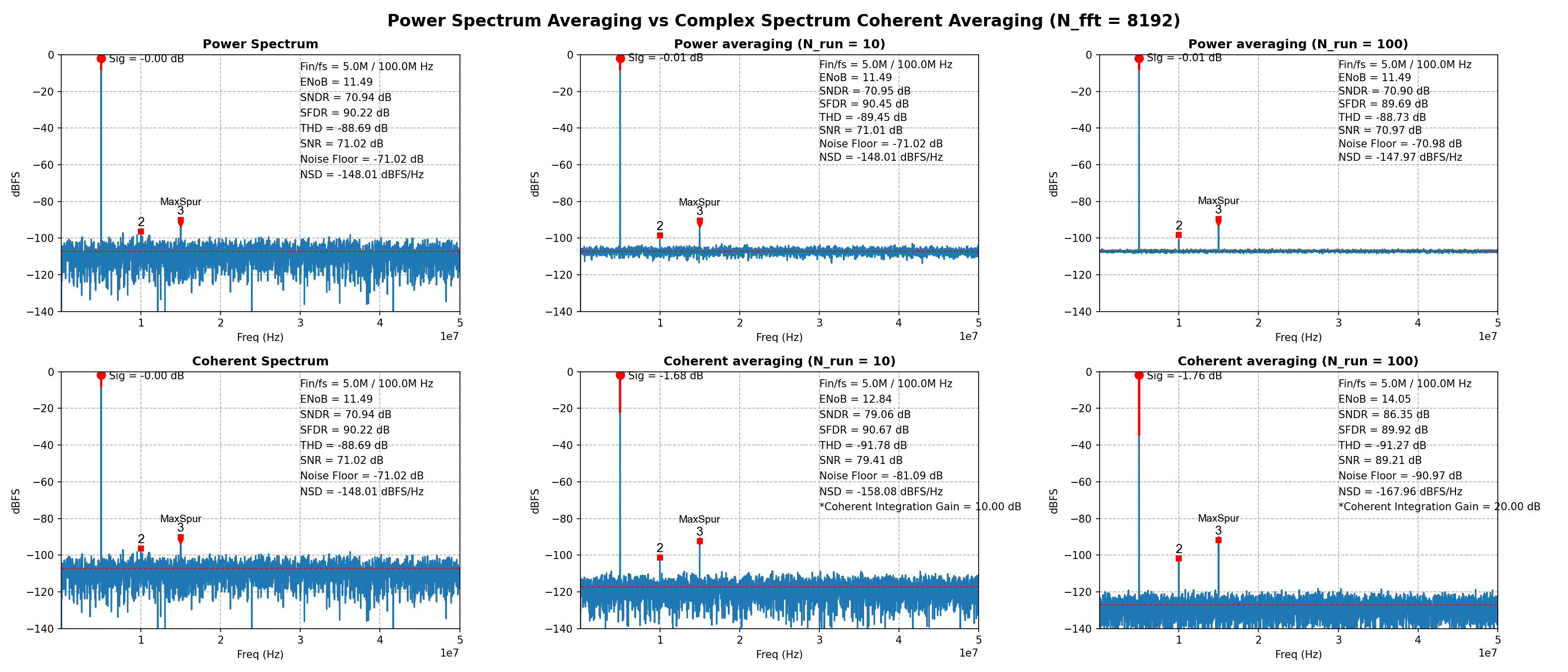
Power averaging vs coherent averaging for noise reduction
exp_s08_windowing_deep_dive.py
Description: Deep dive into window functions for different scenarios.
================================================================================
SCENARIO 1: NON-COHERENT SAMPLING (SPECTRAL LEAKAGE)
================================================================================
[Sinewave] Fs=[100.00 MHz], Fin=[10.00 MHz] (non-coherent), N=[8192], A=[0.500 Vpeak]
[Nonideal] Noise RMS=[50.00 uVrms], Theoretical SNR=[76.99 dB], Theoretical NSD=[-153.98 dBFS/Hz]

Window                     ENoB (b)  SNDR (dB)  SFDR (dB)  SNR (dB)  NSD (dBFS/Hz)
------------------------------------------------------------------------------
Kaiser (beta=38)              12.50      77.03      80.99     77.07        -153.62
Blackman-Harris               12.47      76.84      82.56     76.87        -153.43
Chebyshev (100 dB)            12.38      76.31      82.71     76.33        -152.89
Flat-top                      12.09      74.54       3.76     74.55        -151.11
Blackman                      10.12      62.68       5.01     62.68        -139.23
Hann (raised cosine)           7.55      47.21       5.48     47.21        -123.77
Hamming                        5.74      36.33      12.43     36.33        -112.89
Rectangular (no window)        2.27      15.43      11.18     15.43         -92.11

[Save fig 1/3] -> [D:\ADCToolbox\python\src\adctoolbox\examples\02_spectrum\output\exp_s08_windowing_1_leakage.png]


================================================================================
SCENARIO 2: COHERENT SAMPLING (NO LEAKAGE)
================================================================================
[Sinewave] Fs=[100.00 MHz], Fin=[9.997559 MHz] (coherent, Bin 819), N=[8192], A=[0.500 Vpeak]
[Nonideal] Noise RMS=[50.00 uVrms], Theoretical SNR=[76.99 dB], Theoretical NSD=[-153.98 dBFS/Hz]

Window                     ENoB (b)  SNDR (dB)  SFDR (dB)  SNR (dB)  NSD (dBFS/Hz)
------------------------------------------------------------------------------
Kaiser (beta=38)              12.51      77.05      96.96     77.13        -154.12
Rectangular (no window)       12.51      77.04     103.51     77.06        -154.05
Flat-top                      12.50      77.01      97.48     77.06        -154.05
Blackman-Harris               12.50      76.99      97.70     77.04        -154.03
Blackman                      12.50      76.99      98.01     77.03        -154.03
Hamming                       12.50      76.99      99.67     77.03        -154.02
Hann (raised cosine)          12.50      76.98      99.56     77.02        -154.02
Chebyshev (100 dB)            12.39      76.36      88.80     76.40        -153.39

[Save fig 2/3] -> [D:\ADCToolbox\python\src\adctoolbox\examples\02_spectrum\output\exp_s08_windowing_2_coherent.png]

================================================================================
SCENARIO 3: SHORT FFT (COARSE RESOLUTION)
================================================================================
[Sinewave] Fs=[100.00 MHz], Fin=[10.156250 MHz] (coherent, Bin 13), N=[128], A=[0.500 Vpeak]
[Nonideal] Noise RMS=[50.00 uVrms], Theoretical SNR=[76.99 dB], Theoretical NSD=[-153.98 dBFS/Hz]
[Bin width] = 781.2 kHz (coarse resolution)

[Warning from analyze_spectrum]: Harmonics [2] alias to fundamental (excluded from THD)
Window                     ENoB (b)  SNDR (dB)  SFDR (dB)  SNR (dB)  NSD (dBFS/Hz)
------------------------------------------------------------------------------
Rectangular (no window)       12.50      77.03      84.19     78.39        -155.38
Hamming                       12.34      76.02      80.85     77.91        -154.90
Hann (raised cosine)          12.32      75.94      80.70     77.84        -154.84
Blackman                      12.30      75.79      79.75     79.58        -156.57
Blackman-Harris               12.28      75.71      79.00     82.53        -159.52
Flat-top                      12.24      75.47      78.45     79.01        -156.00
Chebyshev (100 dB)            12.24      75.45      79.62     79.08        -156.07
Kaiser (beta=38)              12.21      75.28      77.55    150.00        -226.99

[Save fig 3/3] -> [D:\ADCToolbox\python\src\adctoolbox\examples\02_spectrum\output\exp_s08_windowing_3_short_fft.png]

================================================================================
SUMMARY: Window Function Selection Rules
================================================================================
1. Non-coherent sampling: Use Kaiser/Blackman-Harris for best leakage suppression
2. Coherent sampling: Simpler windows (Rectangular/Hann/Hamming) work equally well
3. Short FFT: Avoid very wide windows (Kaiser). Use Rectangular/Hann/Hamming
Note: Kaiser window shows SNR=150dB in short FFT scenario - this is a known edge case with very short FFT and wide windows.
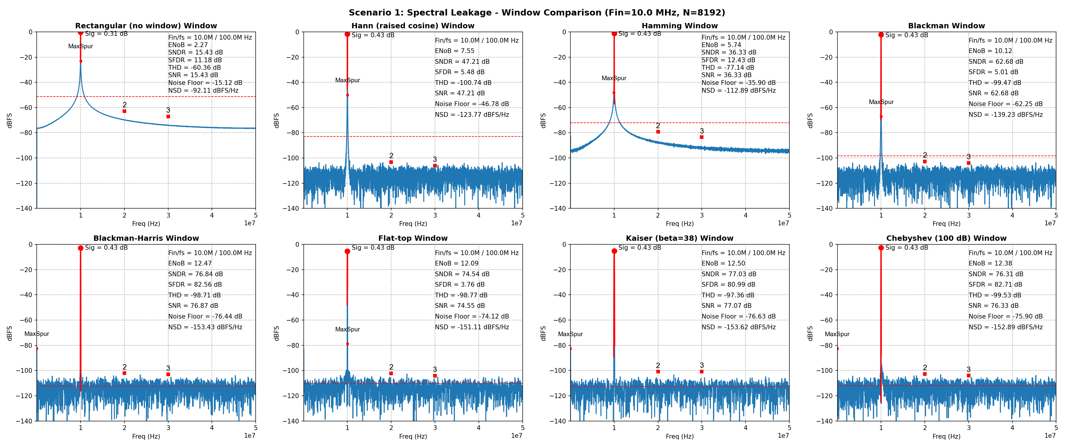
Comparing spectral leakage across different window functions
exp_s10_polar_noise_and_harmonics.py
Description: Polar plot comparison of thermal noise vs harmonic distortion.
[Sinewave] Fs=[800.00 MHz], Fin=[79.98 MHz], Bin/N=[819/8192], A=[0.490 Vpeak]

================================================================================
LEFT: THERMAL NOISE (2 mVrms)
================================================================================
[2 mVrms] SNR=44.8dB → Measured: ENoB=7.13b, SNR=44.72dB

================================================================================
RIGHT: HARMONIC DISTORTION (HD2=-80dB, HD3=-50dB, k3<0)
================================================================================
[HD2=-80dB, HD3=-50dB, k3<0] SNDR=49.07dB, THD=-49.87dB, HD2=-81.22dB, HD3=-49.87dB


[Save fig] -> [D:\ADCToolbox\python\src\adctoolbox\examples\02_spectrum\output\exp_s10_polar_noise_and_harmonics.png]
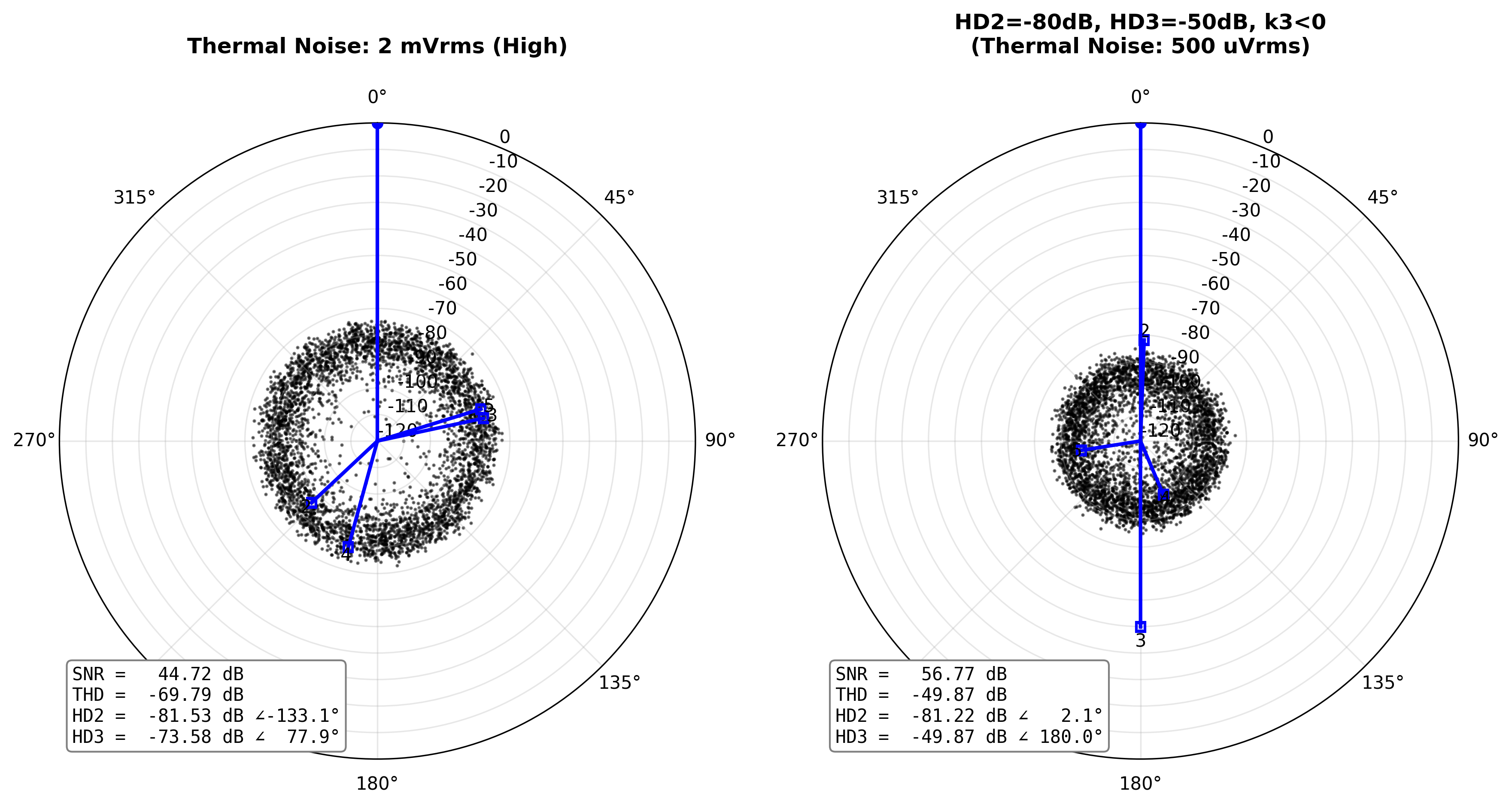
Polar spectrum comparing thermal noise and harmonic distortion
exp_s11_polar_memory_effect.py
Description: Polar plot showing static vs dynamic nonlinearity.
[Sinewave] Fs=[800 MHz], N=[8192], A=[0.490 Vpeak]
[Nonideal] Noise RMS=[50.00 uVrms], Theoretical SNR=[76.81 dB], Theoretical NSD=[-162.83 dBFS/Hz]

================================================================================
ROW 1: STATIC NONLINEARITY
================================================================================
[Fin=79.98 MHz], Bin/N=[819/8192]

[HD3=-66dB, k3>0] SNDR=65.67dB, THD=-66.01dB, HD3=-66.01dB
[HD3=-66dB, k3<0] SNDR=65.64dB, THD=-65.98dB, HD3=-65.98dB
[HD2+HD3] SNDR=65.47dB, THD=-65.81dB, HD2=-79.78dB, HD3=-65.99dB

================================================================================
ROW 2: MEMORY EFFECT
================================================================================
[Fin=   40MHz, ME=0.02] sndr=60.09dB, snr=60.35dB, thd=-72.38dB
[Fin=   80MHz, ME=0.02] sndr=60.06dB, snr=60.33dB, thd=-72.29dB
[Fin=  160MHz, ME=0.02] sndr=59.96dB, snr=60.23dB, thd=-72.19dB


[Save fig] -> [D:\ADCToolbox\python\src\adctoolbox\examples\02_spectrum\output\exp_s11_polar_memory_effect.png]
exp_s12_polar_coherent_averaging.py
Description: Polar plot demonstrating coherent averaging improvement.
[Sinewave] Fs=[100.00 MHz], Fin=[4.980469 MHz] (coherent, Bin 51), N=[1024], A=[0.499 Vpeak]
[Nonideal] Noise RMS=[100.00 uVrms], Theoretical SNR=[70.95 dB], Theoretical NSD=[-147.94 dBFS/Hz]
[Nonlinearity] HD2=[-80 dB], HD3=[-73 dB]

[Generated] 100 runs with random phase

[  1 Run(s)] ENoB=[11.09 b], SNDR=[ 68.55 dB], SNR=[ 71.04 dB]
[ 10 Run(s)] ENoB=[11.61 b], SNDR=[ 71.66 dB], SNR=[ 80.98 dB]
[100 Run(s)] ENoB=[11.69 b], SNDR=[ 72.13 dB], SNR=[ 91.11 dB]

[Save fig] -> [D:\ADCToolbox\python\src\adctoolbox\examples\02_spectrum\output\exp_s12_polar_coherent_averaging.png]
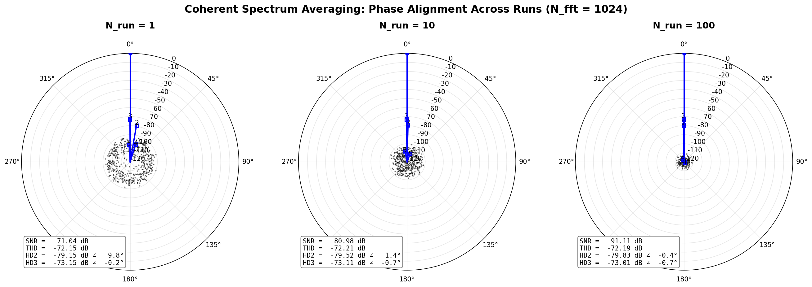
Polar spectrum demonstrating coherent averaging improvement